Lately, as I started learning about Procedural generation, I have been trying to implement the Perlin noise algorithm. Perlin noise is a type of gradient noise that Ken Perlin developed in 1983. Game developers and CG artists usually use it to generate organic looking textures and terrains among many other things.
At its core, the Perlin noise algorithm works in the following way:
- Generate an n-dimensional grid or lattice.
- At each point on the grid, generate a gradient vector. These vectors should be consistent when moving between grid cells. The top right corner of the first cell in a 2D grid should have the exact same vector as the top left corner of the second cell.
- Given an n-dimensional point, find the grid cell to which the point belongs.
- Calculate distance vectors between the point and all of the grid corner.
- Calculate the dot product between each of the distance vectors and its equivalent gradient vector.
- Interpolate between the dot products using a combination of smoothstep and linear interpolation functions.
This is just a quick overview of the algorithm. Here are a few resources that helped me understand how the algorithm works:
- Mountains, Cliffs, and Caves: A Comprehensive Guide to Using Perlin Noise for Procedural Generation
- Perlin noise: What is it, how to use it, and why it’s better than value noise
Naive first implementation
Initially, when I implemented the algorithm, I followed the steps described above literally. The reason I did that was to make sure I actually understood how the algorithm works.
First, I started by calculating a grid using the following code:
#define f32 float
#define i32 int
#define u32 (unsigned int)

#define GRID_LENGTH 64
#define PADDED_GRID_LENGTH (GRID_LENGTH + 2)
#define CELL_SIZE 16
#define CELL_COUNT (PADDED_GRID_LENGTH * PADDED_GRID_LENGTH)

typedef struct {
  f32 x;
  f32 y;
} Vec2;

static const Vec2 gradient_vectors[4] = {
  (Vec2){ 1.0f,  1.0f},
  (Vec2){ 1.0f, -1.0f},
  (Vec2){-1.0f, -1.0f},
  (Vec2){-1.0f,  1.0f}
};

static const Vec2 grid_vectors[CELL_COUNT] = {0};

u32 generate_random_u32(u32 min, u32 max) {
  // using rand() for demonstration purposes only
  return (u32)(rand() % (max - min) + min);
}

void calculate_vectors(void) {
  for (u64 i = 0; i < CELL_COUNT; ++i) {
    grid_vectors[i] = grad_vecs[generate_random_u32(0, 4)];
  }
}Next, I implemented the noise function like this:
f32 fade(f32 t) {
  // smoothstep interpolation function
  return t * t * t * (t * (t * 6 - 15) + 10);
}

f32 lerp(f32 t, f32 a, f32 b) {
  return t * a + (1 - t) * b;
}

void noise_2d(i32 x, i32 y) {
  // NOTE: Vector utilities eliminated for brevity

  i32 cx = x / CELL_SIZE; // x coordinate of grid cell
  i32 cy = y / CELL_SIZE; // y coordinate of grid cell

  f32 x0 = cx       * CELL_SIZE;
  f32 y0 = cy       * CELL_SIZE;
  f32 x1 = (cx + 1) * CELL_SIZE;
  f32 y1 = (cy + 1) * CELL_SIZE;

  // relative position of the point's x coordinate
  f32 xf = (x - x0) / (x1 - x0);
  // relative position of the point's y coordinate
  f32 yf = (y - y0) / (y1 - y0);

  Vec2 p  = {xf, yf};

  Vec2 tl_point = {0.0f, 0.0f}; // top left corner of the grid
  Vec2 tr_point = {1.0f, 0.0f}; // top rigth corner of the grid
  Vec2 bl_point = {0.0f, 1.0f}; // bottom left corner of the grid
  Vec2 br_point = {1.0f, 1.0f}; // bottom right corner of the grid

  // gradient vector of top left corner
  Vec2 tl_vec = grid_vectors[cy       * PADDED_GRID_LENGTH + cx      ];
  // gradient vector of top right corner
  Vec2 tr_vec = grid_vectors[cy       * PADDED_GRID_LENGTH + (cx + 1)];
  // gradient vector of bottom left corner
  Vec2 bl_vec = grid_vectors[(cy + 1) * PADDED_GRID_LENGTH + cx      ];
  // gradient vector of bottom right corner
  Vec2 br_vec = grid_vectors[(cy + 1) * PADDED_GRID_LENGTH + (cx + 1)];

  // distance vector to top left corner
  Vec2 p_tl_vec = vec2_sub(p, tl_point);
  // distance vector to top right corner
  Vec2 p_tr_vec = vec2_sub(p, tr_point);
  // distance vector to bottom left corner
  Vec2 p_bl_vec = vec2_sub(p, bl_point);
  // distance vector to bottom right corner
  Vec2 p_br_vec = vec2_sub(p, br_point);

  f32 tl_dot = vec2_dot(p_tl_vec, tl_vec);
  f32 tr_dot = vec2_dot(p_tr_vec, tr_vec);
  f32 bl_dot = vec2_dot(p_bl_vec, bl_vec);
  f32 br_dot = vec2_dot(p_br_vec, br_vec);

  f32 u = fade(xf);
  f32 v = fade(yf);

  return lerp(u, lerp(v, br_dot, tr_dot), lerp(v, bl_dot, tl_dot));
}Then, I would use these functions in the following way:
int main(void) {
  calculate_vectors();

  for (u32 y = 0; y < 256; ++y) {
    for (u32 x = 0; x < 256; ++x) {
      f32 value = noise_2d(x, y);
      printf("%f\n", value);
    }
  }

  return 0;
}While this implementation successfully generates Perlin noise, it is very inefficient due to the amount of computations it does. However, it proved to me that I at least understand the core idea behind how the algorithm works.
Ken Perlin’s reference implementation
When Ken Perlin published his paper on the improved Perlin noise in 2002, he published a reference implementation of the algorithm alongside it. While, essentially, this reference implementation does the same things described above, it relies on hashing and some bit manipulation tricks to reduce the amount of computations required. Thus, it should perform a lot better than a naive implementation of the algorithm.
However, I had 2 main problems with this reference implementation:
- The implementation is for 3D noise. What I needed was a 2D noise.
- More importantly, I couldn’t map what I learned about the algorithm to the code in the reference implementation.
I could have solved the first problem in a very simple way; just treat every 2D point as a 3D point on the same plane. By passing a constant value for z, I would have essentially got 2D noise. But this means that I would have probably been doing some unnecessary computations. It also means that I would be ignoring the second problem.
Therefore, I had to break down the code to be able to understand it, at least to a certain extent. This is the only way I could solve the two problems since, by understanding the code, I can adapt it to generate 2D noise.
First, here is a C version of the reference implementation:
#include <math.h>

static const i32 permutation[] = {151,160,137,91,90,15,131,13,201,95,96,53,194, 233,
  7,225,140,36,103,30,69,142, 8,99,37,240,21,10,23,190,6,148,247,120,234, 75, 0, 26,
  197, 62,94,252,219,203,117,35,11,32,57,177,33,88,237,149,56,87,174,20,125,136,171,
  168, 68,175,74,165,71,134,139,48,27,166,77,146,158,231,83,111,229,122,60,211, 133,
  230,220,105,92,41,55,46,245,40,244,102,143,54,65,25,63,161,1,216,80,73,209,76,132,
  187,208,89,18,169,200,196,135,130,116,188,159,86,164,100,109,198,173,186,3,64, 52,
  217,226,250,124,123,5,202,38,147,118,126,255,82,85,212,207,206,59,227,47,16,58,17,
  182,189,28,42,223,183,170,213,119,248,152,2,44,154,163,70,221,153,101,155,167, 43,
  172, 9,129,22,39,253,19,98,108,110,79,113,224,232,178,185,112,104,218,246,97, 228,
  251,34,242,193,238,210,144,12,191,179,162,241,81,51,145,235,249,14,239,107,49,192,
  214,31,181,199,106,157,184,84,204,176,115,121,50,45,127,4,150,254,138,236,205, 93,
  222,114,67,29,24,72,243,141,128,195,78,66,215,61,156,180
};

static i32 p[512] = {0};

i32 main(void) {
  for (int i=0; i < 256 ; i++) {
    p[256+i] = p[i] = permutation[i];
  }
}

f32 fade(f32 t) {
  return t * t * t * (t * (t * 6 - 15) + 10);
}

f32 lerp(f32 t, f32 a, f32 b) {
  return a + t * (b - a);
}

f32 grad(i32 hash, f32 x, f32 y, f32 z) {
  i32 h = hash & 15;                      // CONVERT LO 4 BITS OF HASH CODE
  f32 u = h<8 ? x : y,                    // INTO 12 GRADIENT DIRECTIONS.
      v = h<4 ? y : h==12||h==14 ? x : z;
  return ((h&1) == 0 ? u : -u) + ((h&2) == 0 ? v : -v);
}

f32 noise_3d(f32 x, f32 y, f32 z) {
  i32 X  = (i32)floorf(x) & 255,                 // FIND UNIT CUBE THAT
      Y  = (i32)floorf(y) & 255,                 // CONTAINS POINT.
      Z  = (i32)floorf(z) & 255;
      x -= floorf(x);                            // FIND RELATIVE X,Y,Z
      y -= floorf(y);                            // OF POINT IN CUBE.
      z -= floorf(z);
  f32 u  = fade(x),                              // COMPUTE FADE CURVES
      v  = fade(y),                              // FOR EACH OF X,Y,Z.
      w  = fade(z);
  i32 A  = p[X  ]+Y, AA = p[A]+Z, AB = p[A+1]+Z, // HASH COORDINATES OF
      B  = p[X+1]+Y, BA = p[B]+Z, BB = p[B+1]+Z; // THE 8 CUBE CORNERS,

  return lerp(w, lerp(v, lerp(u, grad(p[AA  ], x  , y  , z   ),  // AND ADD
                                 grad(p[BA  ], x-1, y  , z   )), // BLENDED
                         lerp(u, grad(p[AB  ], x  , y-1, z   ),  // RESULTS
                                 grad(p[BB  ], x-1, y-1, z   ))),// FROM  8
                 lerp(v, lerp(u, grad(p[AA+1], x  , y  , z-1 ),  // CORNERS
                                 grad(p[BA+1], x-1, y  , z-1 )), // OF CUBE
                         lerp(u, grad(p[AB+1], x  , y-1, z-1 ),
                                 grad(p[BB+1], x-1, y-1, z-1 ))));
}The permutation table
Instead of generating an actual grid like I did in my naive implementation, Ken uses a permutation table. It wasn’t initially clear to me how this table relates to the grid and how are the the gradient vectors calculated from it. So, let’s break things down and start with a simple example.
Let’s take a look at this 3x3x3 3D grid.
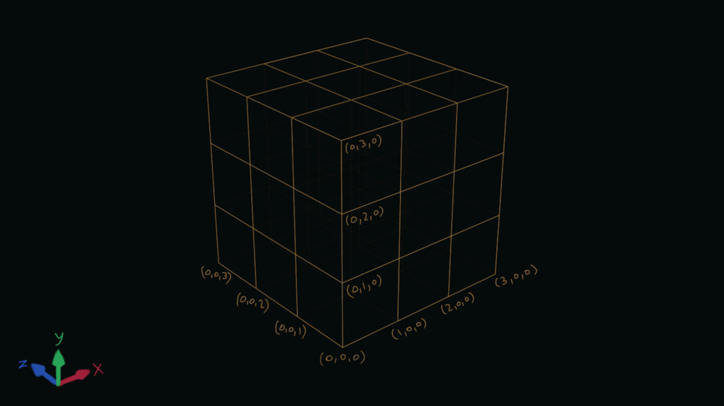
We can imagine this grid as being made of 27 1x1x1 cubes. Each point on this grid has x, y and z coordinates that fall within the range [0..3). This means that a 3D point on the grid is made up of a combination of coordinates that each have one of the values 0, 1 or 2.
But what about the value 3? Why is it not included in the range? The answer to this question is that we want our grid to repeat to get the continuous gradient look of Perlin noise. Any coordinate with the value 3 should wrap around to 0.
If you think about it, you will see that we can represent the possible values for our grid points with a simple array.
static i32 coordinates[] = {0, 1, 2};We then take this array and shuffle its values around to end up with a randomised array of the possible values for the coordinates of the grid points.
This is exactly what Ken does in his implementation, but he uses a 256x256x256 grid instead of a 3x3x3 one. This gives him a randomised table of values in the range [0..256). This is the permutation array in the C implementation of the algorithm.
Optimised permutation table
Ken then proceeds to create another array (called p) that can hold 512 elements. He fills this array with two copies of the permutation array. To my knowledge, this is an optimisation that sacrifices a bit of memory to save on the amount of computations done in the algorithm.
Basically, Ken uses the permutation table to hash the coordinates of each point on the grid cell. For each point, this consists of hashing the value of one coordinate, adding the next one, hasing the result, and so on. Without the repeating permutation table, Ken would have needed to ensure every coordinate is in the range [0..256) by using a modulo (%) operation or a bitwise and (&).
By repeating the table, he can get rid of these extra calculations, making the algorithm more efficient.
Coordinate hashes
The next part that was slightly confusing to me is the coordinate hashes. However, once I broke it down, it became clear how it works. Essentially, it’s a series of hashing and addition operations. If we take a point (x, y, z), then we can hash it in the following way:
// hash is just a pseudo function
u32 h = hash(hash(hash(x) + y) + z);To hash the coordinates of all corners of the cube, we can do it in the following way:
u32 h0 = hash(hash(hash(x  ) + y    ) + z    ); // p[AA  ] in ref implementation
u32 h1 = hash(hash(hash(x+1) + y    ) + z    ); // p[BA  ] in ref implementation
u32 h2 = hash(hash(hash(x  ) + (y+1)) + z    ); // p[AB  ] in ref implementation
u32 h3 = hash(hash(hash(x+1) + (y+1)) + z    ); // p[BB  ] in ref implementation
u32 h4 = hash(hash(hash(x  ) + y    ) + (z+1)); // p[AA+1] in ref implementation
u32 h5 = hash(hash(hash(x+1) + y    ) + (z+1)); // p[BA+1] in ref implementation
u32 h6 = hash(hash(hash(x  ) + (y+1)) + (z+1)); // p[AB+1] in ref implementation
u32 h7 = hash(hash(hash(x+1) + (y+1)) + (z+1)); // p[BB+1] in ref implementationAs you can see, some of the operations are performed multiple times. This is why Ken calculates them separately and saves the results to use them later. This is just another optimisation that saves on the computations that the algorithm does.
The distance vectors
When calling the grad function, Ken calculates the distance vectors between the point and each of the corners of the unit grid cell. He passes the distance vector as a series of coordinates to the function.
Here is a break down how each distance vector relates to one of the grid cell corners.
// AA maps to the corner (0, 0, 0) of the unit cube
// Therefore, distance vector is (x-0, y-0, z-0)
grad(p[AA  ], x  , y  , z   );

// BA maps to the corner (1, 0, 0) of the unit cube
// Therefore, distance vector is (x-1, y-0, z-0)
grad(p[BA  ], x-1, y  , z   );

// AB maps to the corner (0, 1, 0) of the unit cube
// Therefore, distance vector is (x-0, y-1, z-0)
grad(p[AB  ], x  , y-1, z   );

// BB maps to the corner (1, 1, 0) of the unit cube
// Therefore, distance vector is (x-1, y-1, z-0)
grad(p[BB  ], x-1, y-1, z   );

// AA+1 maps to the corner (0, 0, 1) of the unit cube
// Therefore, distance vector is (x-0, y-0, z-1)
grad(p[AA+1], x  , y  , z-1 );

// BA+1 maps to the corner (1, 0, 1) of the unit cube
// Therefore, distance vector is (x-1, y-0, z-1)
grad(p[BA+1], x-1, y  , z-1 );

// AB+1 maps to the corner (0, 1, 1) of the unit cube
// Therefore, distance vector is (x-0, y-1, z-1)
grad(p[AB+1], x  , y-1, z-1 );

// BB+1 maps to the corner (1, 1, 1) of the unit cube
// Therefore, distance vector is (x-1, y-1, z-1)
grad(p[BB+1], x-1, y-1, z-1 );The gradient vectors
The grad function is the part that stumped me the most. I understood the purpose of the function which is to get the gradient vector for one of the cube’s corner and calculate the dot product between it and the distance vector. I also had no problem understanding the code on a technical level since it’s quite simple.
What wasn’t clear to me is the logic behind the code. I couldn’t really wrap my head around why the calculations are done in that manner. I ran the code in the debugger and stepped through it multiple times but couldn’t really connect all the dots together. This is when I turned to ChatGPT.
Side note: This is really one of the good use cases for LLMs. I rarely rely on them to actually implement some code for me, unless it’s a quick thing that I don’t really care about.
However, for trying to brush up on some foundational knowledge or when trying to break down something that I don’t fully understand, I find LLMs to be helpful. Asking the right questions isn’t always easy, especially when digging into an unfamiliar topic. Being able to have a conversation helps a lot. It’s like having a tutor that is available to give me hints that can expand my knowledge.
One of the first parts that weren’t clear to me is the first line of the function
int h = hash & 15; // CONVERT LO 4 BITS OF HASH CODE INTO 12 GRADIENT DIRECTIONS.I knew that the hash & 15 could return 16 possible values. I wasn’t really sure how these values map to only 12 gradient vectors. Additionally, I didn’t even know what are the gradient vectors being used in the function. After some back and forth with ChatGPT, I managed to break this part down and understand what it does.
Mapping the grad outputs to gradient vectors
First, the gradient vectors that result from the calculation above are the vectors that correspond to the 12 edges of the cube. For each edge, we calculate a vector between the center of the cube and the midpoint of the edge. Here is an image illustrating this.
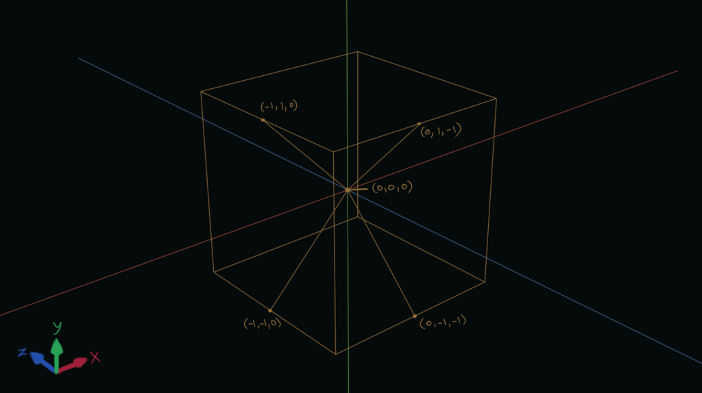
As you can see, we have 4 vectors going from the midpoint of 4 of the cube’s edges to the center of the cube. The center of the cube has the coordinates (0, 0, 0). This means that we end up with the 4 vectors (0, 1, -1), (0, -1, -1), (-1, 1, 0) and (-1, -1, 0). If we end up with the following 12 gradient vectors.
( 1,  1,  0)
( 1, -1,  0)
(-1,  1,  0)
(-1, -1,  0)
( 1,  0,  1)
( 1,  0, -1)
(-1,  0,  1)
(-1,  0, -1)
( 0,  1,  1)
( 0,  1, -1)
( 0, -1,  1)
( 0, -1, -1)The whole of the grad function is designed to get one of these gradient vectors and calculate its dot product with the distance vector. While the hash & 15 returns 16 possible values, 4 of them end up being duplicates of other values. This leaves us with 12 gradient vectors. The following table shows this clearly:
| h value | u source | v source | (h&1) | (h&2) | Gradient vector | Dot product |
|---|---|---|---|---|---|---|
| 0 | x | y | 0 | 0 | (1, 1, 0) | x + y |
| 1 | x | y | 1 | 0 | (−1, 1, 0) | −x + y |
| 2 | x | y | 0 | 1 | (1, −1, 0) | x − y |
| 3 | x | y | 1 | 1 | (−1, −1, 0) | −x − y |
| 4 | x | z | 0 | 0 | (1, 0, 1) | x + z |
| 5 | x | z | 1 | 0 | (−1, 0, 1) | −x + z |
| 6 | x | z | 0 | 1 | (1, 0, −1) | x − z |
| 7 | x | z | 1 | 1 | (−1, 0, −1) | −x − z |
| 8 | y | z | 0 | 0 | (0, 1, 1) | y + z |
| 9 | y | z | 1 | 0 | (0, −1, 1) | −y + z |
| 10 | y | z | 0 | 1 | (0, 1, −1) | y − z |
| 11 | y | z | 1 | 1 | (0, −1, −1) | −y − z |
| 12 | y | x | 0 | 0 | (1, 1, 0) dupe of h=0 | y + x |
| 13 | y | x | 1 | 0 | (−1, 1, 0) dupe of h=1 | −y + x |
| 14 | y | x | 0 | 1 | (1, −1, 0) dupe of h=2 | y − x |
| 15 | y | x | 1 | 1 | (−1, −1, 0) dupe of h=3 | −y − x |
For each corner of the cube, the grad function returns the value of the dot product.
Second implementation
Armed with my new understanding of the reference implementation, I decided to revisit my 2D noise version of the algorithm. In 2D, we only need 4 gradient vectors. Similar to the 3D reference implementation, I chose vectors that go from the center of the unit square to the midpoints of each of its edges. This results in the following vectors:
( 1,  0)
(-1,  0)
( 0,  1)
( 0, -1)To get one of these vectors and calculate the dot product for each of the square’s corners, this is the function I use:
f32 gradient_vector_2d(u32 hash, f32 x, f32 y) {
  u32 h = hash & 3;
  if (h == 0) {
    // gradient vector is (1, 0)
    // (1, 0) . (x, y) = x + 0 = x
    return  x;
  }

  if (h == 1) {
    // gradient vector is (-1, 0)
    // (-1, 0) . (x, y) = -x + 0 = -x
    return -x;
  }

  if (h == 2) {
    // gradient vector is (0, 1)
    // (0, 1) . (x, y) = 0 + y = y
    return  y;
  }

  // gradient vector is (0, -1)
  // (0, -1) . (x, y) = 0 - y = -y
  return -y;
}And this is the implementation of the noise function itself. As you can see, I use a permutation table that is double the size of the one Ken Perlin used.
#define PERMUTATION_COUNT 512

u32 generate_random_u32(u32 min, u32 max) {
  // using rand() for demonstration purposes only
  return (u32)(rand() % (max - min) + min);
}

void shuffle(u32 *array, u32 count) {
  u32 j;
  u32 tmp;
  for (u32 i = count - 1; i >= 1; --i) {
    j        = generate_random_u32(0, i);
    tmp      = array[i];
    array[i] = array[j];
    array[j] = tmp;
  }
}

i32 main(void) {
  // fill temp array with indices
  u32 tmp[PERMUTATION_COUNT] = {};
  for (u32 i = 0; i < PERMUTATION_COUNT; ++i) { tmp[i] = i; }

  shuffle(tmp, PERMUTATION_COUNT);

  // fill the permutations table
  for (u32 i = 0; i < PERMUTATION_COUNT; ++i) {
    perlin_permutations[i] = perlin_permutations[PERMUTATION_COUNT + i] = tmp[i];
  }
}

f32 perlin_noise_2d(f32 x, f32 y) {
  f32 fx = floorf(x);
  f32 fy = floorf(y);

  u32 xu = (u32)fx & (PERMUTATION_COUNT - 1);
  u32 yu = (u32)fy & (PERMUTATION_COUNT - 1);

  x -= fx;
  y -= fy;

  u32 a = perlin_permutations[xu    ] + yu;
  u32 b = perlin_permutations[xu + 1] + yu;

  f32 u = fade(x);
  f32 v = fade(y);

  return lerp(v, lerp(u, gradient_vector_2d(perlin_permutations[a    ], x    , y    ),
                         gradient_vector_2d(perlin_permutations[b    ], x - 1, y    )),
                 lerp(u, gradient_vector_2d(perlin_permutations[a + 1], x    , y - 1),
                         gradient_vector_2d(perlin_permutations[b + 1], x - 1, y - 1)));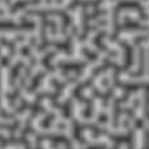
}Using this function, I could generate 2D Perlin noise textures like the one below.